OpenTelemetry Histograms with Prometheus

Histograms record the distribution of a measurement like latency and are used to compute percentiles on them. It divides the entire range of measurements into a set of buckets and counts how many values fall into each bucket. OpenTelemetry has support for two types of histograms:

Explicit Bucket Histogram

As the name implies, the buckets are explicitly defined at the time of initialization. The OpenTelemetry agents have a default set of buckets defined. For e.g. the Java agent uses these buckets by default:

0, 5, 10, 25, 50, 75, 100, 250, 500, 750, 1_000, 2_500, 5_000, 7_500, 10_000, ∞.

These values correspond to measurements in milliseconds when used for latency.

While this is a reasonable default, it doesn’t work well in all scenarios. For example, a low-latency trading platform might have values in the microseconds to milliseconds range, whereas a 3rd party API call could range from hundreds of milliseconds to a few seconds. This could lead to data being concentrated in a few of the limited buckets resulting in erroneous percentile values.

Customizing the buckets is NOT a simple configuration change, and depending on the OpenTelemetry agent used, this would require either a code change or deploying an agent extension.

Customize Histogram Buckets

Asserts uses a Prometheus-compatible time series database. Recently a customer of ours ran into an issue that required customizing the buckets. This customer is in the fintech domain, and a service of theirs integrates with a number of external APIs of other financial institutions. These APIs, at times, take well beyond 10 seconds. What we noticed in the Asserts KPI dashboard is that while the average latency is well beyond 30 seconds, the P99 reported is maxed at 10 seconds, which was incorrect:

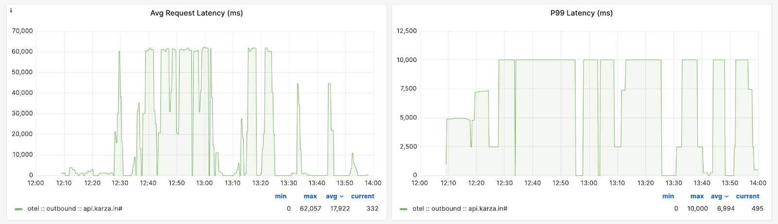
The default buckets don’t sufficiently capture the distribution of the latencies in this case. As explained in an earlier blog post, the fix for this is to add more buckets above 10 seconds to the histogram. OpenTelemetry has a newer exponential bucket histogram metric, which could have addressed this, but we couldn't use it as the metrics are exported using a Prometheus exporter, and that doesn't support the exponential bucket histogram yet—more about this later in the blog.

OpenTelemetry Java agent, which was used to instrument this service, doesn’t provide a configuration to define the custom buckets. As suggested here, the agent SDK provides a mechanism to define views using which we can configure how measurements are aggregated and exported as metrics. Views can be used to configure bucket boundaries, as explained in the Javadoc for SdkMeterProviderBuilder::register method. This needs to be packaged as a Java agent extension. Another alternative is to use the experimental view file configuration module.

The OpenTelemetry Java Agent Instrumentation project has a few examples that demonstrate how to create an extension. The extensions can be added to the JVM using the system property ‘otel.javaagent.extensions’. Following the sample extensions, here’s a simple class that configures custom histogram bucket ranges:

@AutoService(AutoConfigurationCustomizerProvider.class)
public class HistogramBucketConfig implements AutoConfigurationCustomizerProvider {


   private static final List<Double> DEFAULT_HISTOGRAM_BUCKET_BOUNDARIES =
           Collections.unmodifiableList(
                   Arrays.asList(
                           0d, 5d, 10d, 25d, 50d, 75d, 100d, 250d, 500d, 750d, 1_000d, 2_500d, 5_000d, 7_500d,
                           10_000d, 30_000d, 60_000d, 90_000d, 120_000d));


   @Override
   public void customize(AutoConfigurationCustomizer autoConfiguration) {
       autoConfiguration.addMeterProviderCustomizer(
               (sdkMeterProviderBuilder, configProperties) ->
                       sdkMeterProviderBuilder.registerView(
                               InstrumentSelector.builder()
                                       .setName("*duration")
                                       .setType(InstrumentType.HISTOGRAM)
                                       .build(),
                               View.builder()
                                       .setAggregation(
                                               Aggregation.explicitBucketHistogram(DEFAULT_HISTOGRAM_BUCKET_BOUNDARIES))
                                       .build()));
   }
}

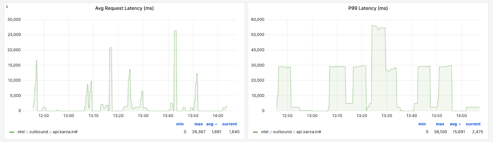
The complete source code for this is available on github. With this change in place, P99 latencies are now accurately captured:

Shortcomings of Explicit Bucket Histogram

Even with customization, it’s unlikely for the buckets to be optimally defined for all the different APIs observed in the service.

Besides, when used with a metric store like Prometheus, each bucket is stored as a separate time series. A histogram with N buckets results in N+2 times series when stored in Prometheus (the 2 additional time series are for sum and count)

What if we could do away completely with the need to define bucket ranges, choose bucket ranges accurately based on the range of the observed data, and at the same cost as the earlier histogram? That’s exactly what the new Exponential Histogram offers.

Exponential Histogram

'Exponential Histogram' does away with the need to configure buckets by defining the bucket ranges using an exponential scale. The scale factor is chosen based on the range of input values and controls the resolution of the buckets. Let’s look at a few examples to demystify this:

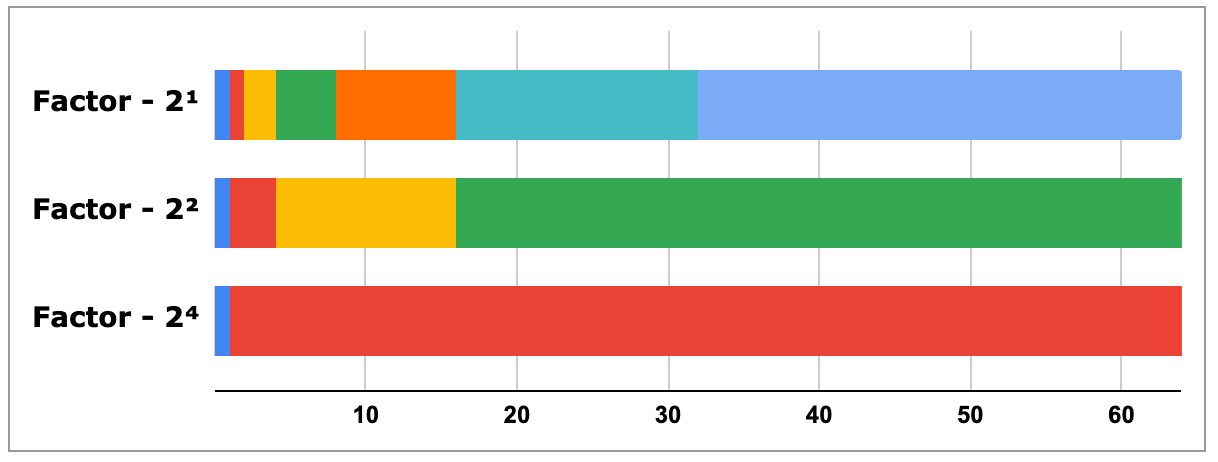
With a factor of 2¹, the buckets are defined as

Increasing the factor lowers the bucket resolution (i.e. wider buckets):

Decreasing the factor increases the bucket resolution (i.e. narrower buckets):

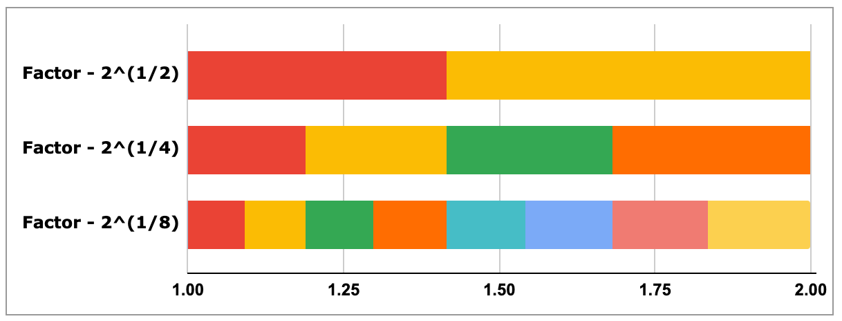
By adjusting the factor, the histogram can accurately capture a wide range of distributions, be it from 1ms - 4ms range or 1ms - 1min range. The reason why the factor is a 2 to the power ± n is it gives it a perfect-subsetting property that allows the merging of a high-resolution histogram with a lower-resolution histogram.

The encoding of this histogram is also more compact, allowing it to be more efficiently transferred over the wire and stored in a backend like Prometheus.

Prometheus Native Histogram

In the near future, we can expect to see end-to-end support for OpenTelemetry Exponential Histograms in Prometheus with Native Histograms. This is available as an experimental feature in Prometheus v2.40. This is a very exciting development, as we can get 10X more precision at an even lower cost than classic Histograms, as outlined in this talk.

OpenTelemetry's exponential bucket histogram can be mapped to this 'Native Histogram.' Presently, only the Prometheus remote write exporter for the OpenTelemetry collector can write these histograms to Prometheus, as explained in this talk.  

We should expect to see wider adoption of exponential histograms in the Prometheus ecosystem once we have the following pieces in place:

• Native histograms to be made available as a stable feature in Prometheus
• A text format to be defined for native histograms by Prometheus. This is a pre-requisite for adding support to the Prometheus exporter in OpenTelemetry agents, as explained here.
• Support for Native Histograms by other popular Prometheus-compatible stores like VictoriaMetrics and Grafana Mimir