Introduction

Prometheus has four metric types, among which the two basic ones are counter and gauge. A gauge is intuitive as it matches our expectation for a metric, i.e., it represents a numeric value that measures something like temperature, memory usage, etc. A counter that monotonically increases, on the other hand, is not so intuitive.

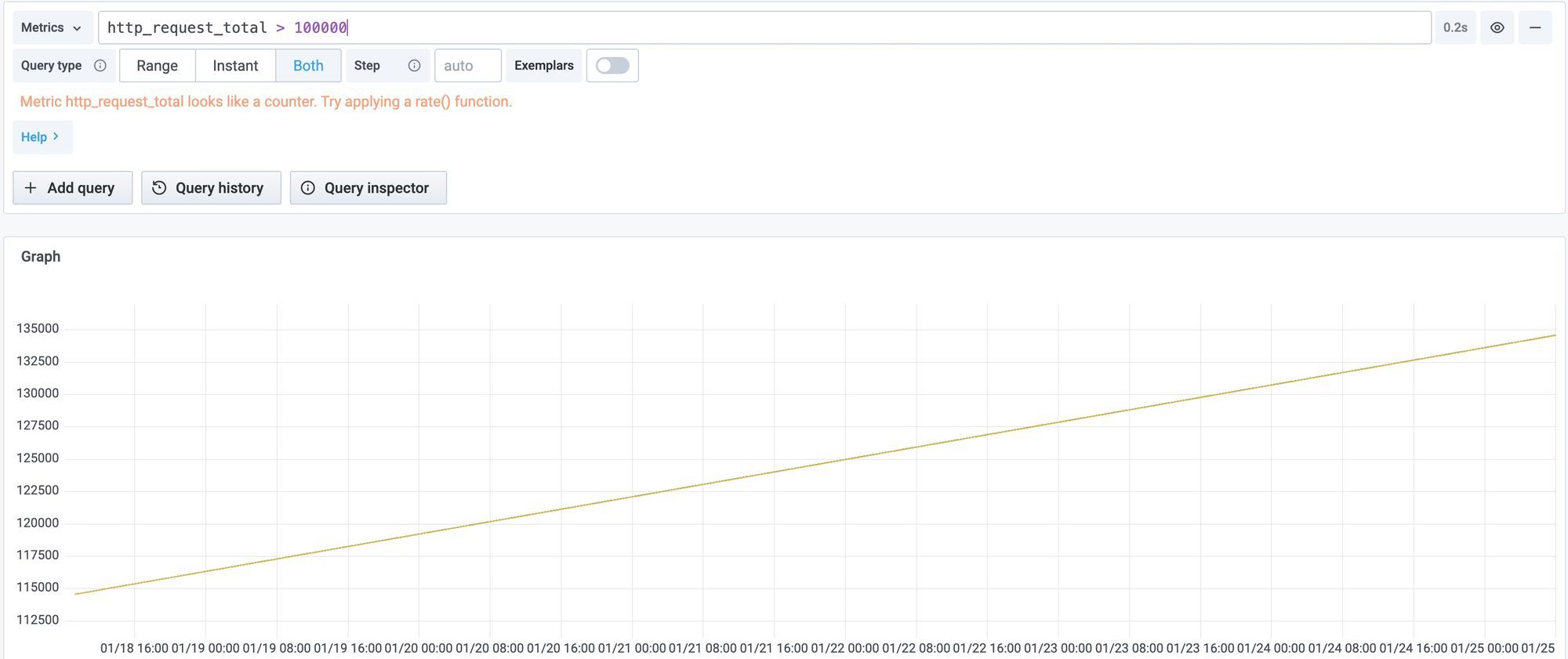
When you start to query counters, you will immediately notice that you always need to apply the rate() function to make use of them. Grafana even tries to remind you that.

So you have to write the following expression to get the request rate:

rate(http_request_total[5m])

For latency, you need to write an even longer expression:

rate(http_request_duration_microseconds_sum[5m])
/
rate(http_request_duration_microseconds_count[5m])

If you are new to Prometheus, this surely seems a bit strange. So why does the metric system record totals that are useless on their own instead of the actual request rate and latency?

In this blog, we will try to answer this question and explain why we recommend using Prometheus counters for your monitoring solution.

Background

As we know, a monitoring system usually comprises clients and servers. Clients collect metrics on monitored software or hardware components. Servers collect metrics from clients and do aggregation across clients and time. The client-server communication can be either a push from the client or a pull from the server.

If a client records the calculated rate or latency, it’s essentially reporting a gauge. We often cannot aggregate gauges. For example, if a service has two instances, at a particular minute, suppose one reports an average latency of 100ms and the other reports 200ms. We cannot average these two numbers and say the average latency for the service at this minute is 150ms, as each instance may be processing different numbers of requests. Similarly, if we want to get the average latency for an hour, we cannot average the latency reported at each minute during the hour.

For this reason, most monitoring solutions make clients record latency totals and request totals as counters. The server will collect from all clients then aggregate totals to calculate rate/latency. After each server collection, the clients reset these counters to 0, ready for the next cycle. StatsD counters are one such example.

With a push model, this has an obvious downside: if the push fails, we lose the value in that time. With a pull model, there is an additional problem. If we reset the counter at each pull, we can only have one server scraping its value because if we have more than one, each server will only get a slice of the increments. There goes our high availability.

Prometheus counters

Prometheus evolves the counter approach a little more. It chooses to have its counters monotonically increasing until the client has to restart. The client never resets the counters. As it turns out, this design has a few crucial benefits.

First of all, it simplifies the clients. All a client does is increment a counter for each event occurrence. It does no other calculation.

Secondly, it is more fault-tolerant. If a scrape fails, the next one still gets all the increments. We only lost the resolution in between. If we want redundancy for availability, we can have two servers scraping from the same client, and they both get the full increments.

Thirdly, the client does not care about the flush interval and thus maintains the raw data with the finest granularity. For data consumers, the server’s scrape interval decides the granularity, but it is usually much easier to update the server configuration than to update the clients. Hence, Prometheus provides more flexibility for granularity.

Lastly, and perhaps the most important benefit is that Prometheus counters can be aggregated across any label combinations and arbitrary time ranges.

For example, if we need to know the request rate for each job, we can do:

sum by (job) (rate(http_request_total[5m]))

If we need to know the request rate on each URL endpoint for a particular job, we can do:

sum by (url) (rate(http_request_total{job=”foo”}[5m]))

Such flexibility is even more important if we are analyzing metrics involving divisions. For average latency for each job, we can write:

sum by (job) (rate(http_request_duration_microseconds_sum[5m])) 
/ 
sum by (job) (rate(http_request_duration_microseconds_count[5m]))

For the server error ratio, we can write:

sum by (job) (rate(http_request_total{status_code=”5.*”}}[1h]))
/
sum by (job) (rate(http_request_total[1h]))

Other monitoring solutions that use gauges or reset-at-flush counters do not have similar flexibility. Their aggregation usually has fixed time ranges and predefined dimensions.

Prometheus counters also serve as the foundation for the other two metric types: summary metrics are essentially two counters, and histogram metrics are recorded as counters for a set of observation buckets. In the monitoring industry, aggregatable histograms have always been a challenge. By counting requests for each performance bucket, Prometheus gives its user the option to slice and dice the histogram on any label combinations. For instance, the following example calculates the P99 latency for each job. If you want to calculate P99 for each URL endpoint, simply add URL to the by clause.

histogram_quantile (
   0.99,
   sum(rate(http_server_requests_seconds_bucket[1m]) > 0) by (le, job)
)

Surely this histogram approach comes with considerable overhead, but it does give users a lot of flexibility.

Trade-off

While the client implementation is greatly simplified, some complexity falls on the server. In particular, how to handle the case when the client restarts and the counter resets to 0?

Prometheus’s rate() function automatically handles it by extrapolation. Without going into the details, we can assume that it detects counter decrease and extrapolate the rate in-between, which, however, implies that:

• The implementation of rate() can not directly use the difference between the start value and the end value. It needs to go through all the samples in the time range. When the range is wide, rate() can become an expensive query.
• Counterintuitively, the changes() function is a syntax sugar on top of rate(), not based on the difference between start and end, thus is subject to the same extrapolation cost.
• It’s usually a bad idea to directly aggregate counters. If we want to summarize rates, we have to calculate rates before adding them up, instead of applying rate() on the sum of counters. This principle is called rate-then-sum.

Besides these nuances, the actual implementation of the rate() function has its well-known intricacy and controversy, though that’s beyond the scope of this short blog.